Fitting a sigmoid curve in R

by Kyriakos Chatzidimitriou | Jul 8, 2012 08:54 | tutorials

rsigmoid

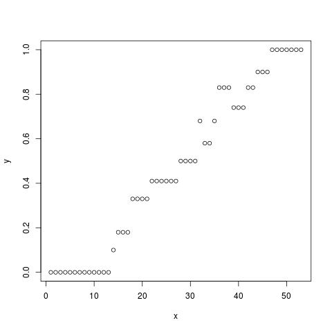
This is a short tutorial on how to fit data points that look like a sigmoid curve using the nls function in R. Let’s assume you have a vector of points you think they fit in a sigmoid curve like the ones in the figure below.

points

The general form of the logistic or sigmoid function is defined as:

$y(x) = A + \frac{K-A}{(1+Qe^{-B(t-M)})^{1/\nu}}$

Let’s assume a more simple form in which only three of the parameters K, B and M, are used. Those are the upper asymptote, growth rate and the time of maximum growth respectively.

$y(x) = \frac{K}{1+e^{-B(t-M)}}$

The following R code estimates the parameters, where y is a vector of data points:

# function needed for visualization purposes
sigmoid = function(params, x) {
  params[1] / (1 + exp(-params[2] * (x - params[3])))
}
    
x = 1:53
y = c(0,0,0,0,0,0,0,0,0,0,0,0,0,0.1,0.18,0.18,0.18,0.33,0.33,0.33,0.33,0.41,
  0.41,0.41,0.41,0.41,0.41,0.5,0.5,0.5,0.5,0.68,0.58,0.58,0.68,0.83,0.83,0.83,
  0.74,0.74,0.74,0.83,0.83,0.9,0.9,0.9,1,1,1,1,1,1,1)
    
# fitting code
fitmodel <- nls(y~a/(1 + exp(-b * (x-c))), start=list(a=1,b=.5,c=25))
    
# visualization code
# get the coefficients using the coef function
params=coef(fitmodel)
    
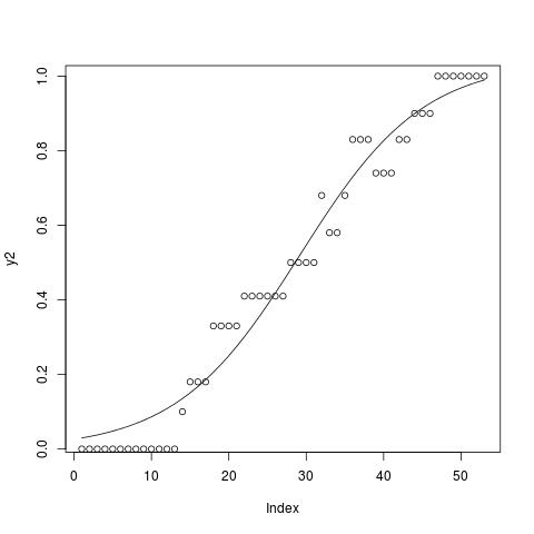
y2 <- sigmoid(params,x)
plot(y2,type="l")
points(y)

Now the data points along with the sigmoid curve look like this, with a = 1.0395204, b = 0.1253769, and c = 29.1724838.

prediction