Modified Gombertz and Baranyi equations are two of the most famous equations for modelling bacterial growth. Bacterial growth is modelled in four different phases:

• The lag phase
• The log or exponential phase
• The stationary phase
• The death phase

Researchers in the food engineering industry are interested in the first two (or three) phases, since in order to maintain low bacterial populations you are interested in prolonging the initial phase and prohibiting the growth of the population. In the first three phases the growth curves resemble what is called a sigmoid curve. As in a previous blog post on fitting sigmoid curves using R I will use the non-linear least-squares method in R to fit these specific curve into the data.

Both the data and the equations are taken from the edited book of McKellar and Lu, 2004: Modeling Microbial Response in Food.

Modified Gompertz

The modified Gompertz equation is equation (2.2) from the book and is given as:

$log(x_t) = A + C \cdot e^{-e^{(-B \cdot (t - M))}}$

where $x_t$ is the number of cells at time $t$, $A$ the asymptotic count, $C$ the difference in value of the upper and lower asymptote, $B$ the relative growth rate at $M$, and $M$ the time at which the absolute growth rate is maximum.

Some data from the book for Listeria monocytogenes at 5 degrees Celsius are:

# time in days
d = c(0, 6, 24, 30, 48, 54, 72, 78, 99, 126, 144, 150, 168, 174, 191, 198, 216, 239, 266, 291, 316, 336, 342, 360, 384)
# log cfu ml^-1
y = c(4.8, 4.7, 4.7, 4.7, 4.9, 5.1, 5.3, 5.4, 5.9, 6.3, 6.9, 6.9, 7.2, 7.3, 7.7, 7.8, 8.3, 8.8, 9.1, 9.2, 9.3, 9.7, 9.7, 9.7, 9.5)

Let's start with defining the Gompertz equation in R:

gombertz_mod = function(params, x) {
  params[1] + (params[3] * exp(-exp(-params[2] * (x - params[4]))))
}

Next I fit the model using non-linear least squares

fitmodel <- nls(y ~ A + C * exp(-exp(-B * (d - M))), start=list(A=3, B=0.01, C=10, M=10))

Extract the parameters and apply the model to new data

gomb_params=coef(fitmodel)
print(gomb_params)

##            A            B            C            M 
##   4.65920718   0.01163221   5.40581821 138.91015307

d2 <- 0:400
y2 <- gombertz_mod(gomb_params, d2)
y_pred_gomb <- gombertz_mod(gomb_params, d)

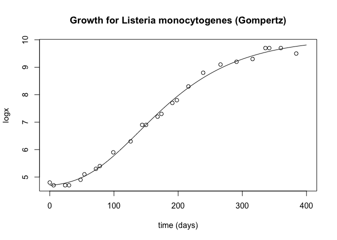
Let's plot the equations and the data points:

plot(d2, y2, type="l", xlab="time (days)", ylab="logx", main="Growth for Listeria monocytogenes (Gompertz)")
points(d, y)

and calculate the RMSE:

rmse <- function(real, pred) {
  sqrt(mean((real-pred)^2))
}

paste("RMSE modified Gombertz: ", rmse(y, y_pred_gomb))

## [1] "RMSE modified Gombertz:  0.112256060122191"

Baranyi

The Baranyi, equations (2.9) and (2.10) from the book are:

$y(t) = y_0 + \mu_{max} \cdot A(t) - ln(1 + \frac{e^{\mu_{max} \cdot A(t)} - 1}{e^{y_{max}-y_0}})$

and

$A(t) = t + \frac{1}{\mu_{max}} \cdot ln(e^{-\mu_{max} \cdot t} + e^{-\mu_{max} \cdot \lambda} - e^{[-\mu_{max} \cdot (t + \lambda)]})$

where $y(t)=lnx(t)$, $y_0=lnx_0$, $\mu_{max}$ is the rate of increase of the limiting substrate and $\lambda$ is the lag-phase duration. Note: the equation for $A_(t)$ is derived after substituting $q_0$ with $\frac{1}{e^{\mu_{max}} - 1}$ in the original equation from the book.

Thus in R for the Baranyi model, we have the following function:

fitmodel <- nls(y ~ y0 + mmax * (d + (1/mmax) * log(exp(-mmax*d) + 
                exp(-mmax * lambda) - exp(-mmax * (d + lambda)))) - 
                log(1 + ((exp(mmax * (d + (1/mmax) * log(exp(-mmax*d) +
                exp(-mmax * lambda) - exp(-mmax * 
                (d + lambda)))))-1)/(exp(ymax-y0)))),
                start=list(y0=2.5, mmax=0.1, lambda=10, ymax=10))

baranyi <- function(params, x) {
  params[1] + params[2] * (x + (1/params[2]) * log(exp(-params[2]*x) + 
  exp(-params[2] * params[3]) - exp(-params[2] * (x + params[3])))) - 
  log(1 + ((exp(params[2] * (x + (1/params[2]) * log(exp(-params[2]*x) + 
  exp(-params[2] * params[3]) - exp(-params[2] * (x + params[3])))))-1)/
    (exp(params[4]-params[1]))))
}

baranyi_params <- coef(fitmodel)
print(baranyi_params)

##          y0        mmax      lambda        ymax 
##  4.63245864  0.02577884 65.17090445  9.69155419

d3 <- 0:400
y3 <- baranyi(baranyi_params, d3)
y_pred_baranyi <- baranyi(baranyi_params, d)

plot(d3, y3, type="l", xlab="time (days)", ylab="logN", main="Growth for Listeria monocytogenes (Baranyi)")
points(d, y)

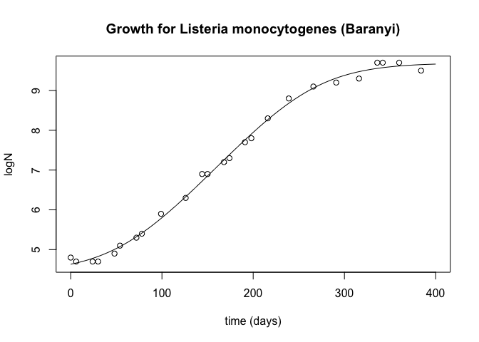
paste("RMSE Baranyi: ", rmse(y, y_pred_baranyi))

## [1] "RMSE Baranyi:  0.102942076757872"

As expected from the bibliography, the Baranyi equations have a smaller error, basically due to the better fit in the steady state of the bacterial growth.

A rendered edition of the R markdown notebook can be found in Rpubs.