This is the first paper review, in a series of paper reviews and implementations I would like to do, on online (or streaming) outlier detection algorithms. I believe with the advent of the Internet of Things it will be an important subject to research and study with all the sensory data to be produced and consumed. All the knowledge from this series will be gathered in the awesome-streaming-outlier-detection repository.

In this first post in the series I am going to present the 2005 paper: Data Outlier Detection using the Chebyshev Theorem by Brett G. Amidan, Thomas A. Ferryman, and Scott K. Cooley.

The paper uses the Chebyshev inequality in order to calculate upper and lower outlier detection limits. These thresholds give a bound to the percentage of data that fall ouside k standard deviations from the mean, while on the same time, the calculations make no assumptions about the distribution of the data. This is important as often the distribution is not known and we don't want to make any assumption over it. The only assumptions the method makes is that the data are independent measurements and that only a small percentage of the outliers are contained in the data.

With an unknown distribution, the Chebysev inequality is:

$P(|X - \mu| \leq k \sigma) \geq (1 - \frac{1}{k^2})$ (1)

and indicates that if k=2 at least 75% of the data would fall within 2 standard deviations from the mean (lower bound). The equation above can also be changed as:

$P(|X - \mu| \geq k \sigma) \leq \frac{1}{k^2}$ (2)

to indicate that at most 25% of the data is outside 2 standard deviations from the mean (upper bound).

There is also a special case when, if we assume that the data is unimodal, (data with only one peak, which can be examined for example by plotting the data) we can use the unimodal Chebyshev's inequality. But since we are talking about streaming data that arrive one after the other, I will assume that nothing is known in advance and continue with the standard case.

From the Chebyshev's inequality an Outlier Detection Value (ODV) is calculated. Any data value that is more extreme than the ODV is considered to be an outlier.

The algorithm

The algorithm follows a two stage process.

Stage 1

The first stage is responsible for trimming the data from values that are possibly outliers.

1. We decide on a value of $p_1$, which can be considered as the probability of seeing an expected outlier. We can use values like 0.1, 0.05 or even 0.01.
2. Solving equation (2) for k we have equation (3). Anything more extreme than k standard deviations is considered a stage-1 outlier. So if $p_1=0.05$ then $k=4.472$ and thus everything more extreme than 4.472 standard deviations will be considered a stage-1 outlier.

$k=\frac{1}{\sqrt{p_1}}$ (3)

3. Then we calculate ODVs (upper and lower bounds) for stage-1, where $\mu$ and $\sigma$ are the sample mean and the sample standard deviation derived from the data:

$ODV_{1U} = \mu + k \sigma$ (4)

$ODV_{1L} = \mu - k \sigma$ (5)

Data that are more extreme than the ODVs of stage-1 are removed from the data for the second phase of the algorithm. The truncated dataset (i.e. without the outliers) is used to calculate the mean and standard deviation needed for the Chebyshev's inequality.

Stage 2

The second stage derives the final ODVs.

1. Select a value for $p_2$, the expected probability of seeing an outlier. Usually smaller than $p_1$, used to actually determine the outliers. Reasonable values are 0.01, 0.001, 0.0001.
2. Solve equation (2) for k and get equation (6).

$k=\frac{1}{\sqrt{p_2}}$ (6)

3. Calculate stage-2 ODVs using equations (4) and (5), where $\mu$ and $\sigma$ are the sample mean and the sample standard deviation derived from the truncated data.
4. All data (from the complete dataset) that are more extreme than the stage-2 ODVs are considered to be outliers.

Streaming version

Even though the algorithm is not made for streaming data, I will convert it into a streaming algorithm by calculating the running average and variance of the data using Welford's online algorithm and benchmark it using the Numenta Anomaly Benchmark (NAB).

The code for the algorithm can be found in my personal fork of the NAB GitHub repository. It achieves:

• 18.44 in the Standard Profile
• 13.18 Reward Low FP
• 23.21 Reward Low FN

with 100.00 being the perfect score in all three categories. Even though the score maybe low, every record is handled in constant time O(1) and there are no assumptions made whatsoever regarding the distribution of the incoming data.

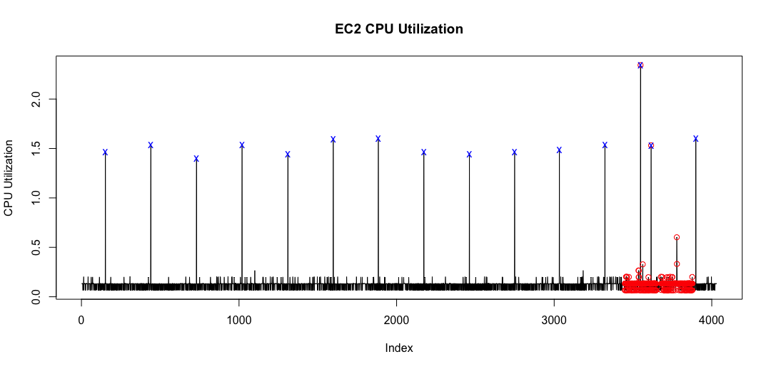
Below is an example of outliers detected from a time series of AWS EC2 CPU utilization:

With red circles we have the points labeled as outliers, while with blue crosses are the predicted ones. As one can see the algorithm is capable of identifying unique outliers rather than periods of "outlierish" behavior needed by NAB.

The code for the NAB implementation can be found below:

from nab.detectors.base import AnomalyDetector

import math

class ChebyshevDetector(AnomalyDetector):
    """ An streaming version of the algorithm found in the paper: 
    "Data Outlier Detection using the Chebyshev Theorem"
    using Welford's online algorithm to calculate mean and standard deviation
    """

    def __init__(self, *args, **kwargs):
        super(ChebyshevDetector, self).__init__(*args, **kwargs)
        self.p1 = 0.1 # Stage 1 probability 
        self.p2 = 0.001 # Stage 2 probability 
        self.k1 = 1/math.sqrt(self.p1)
        self.k2 = 1/math.sqrt(self.p2)
        self.n1 = 0
        self.m1 = 0
        self.m1_2 = 0
        self.std1 = 1
        self.n2 = 0
        self.m2 = 0
        self.m2_2 = 0
        self.std2 = 1

    def handleRecord(self, inputData):
        """Returns a tuple (anomalyScore).
        The input value is considered an outlier if it resides outside the Outlier Detection Values (upper or lower).
        The anomalyScore is calculated based on the normalized distance the input value has from the upper or lower 
        ODVs, if the input value is considered and outlier, otherwise it is 0.0.
        The probabilities p1 and p2 have been tuned a bit to give good performance on NAB.
        """
        anomalyScore = 0.0
        inputValue = inputData["value"]
        # stage 1 statistics
        self.n1 += 1
        delta = inputValue - self.m1
        self.m1 += delta/self.n1
        self.m1_2 += delta * (inputValue - self.m1)
        self.std1 = math.sqrt(self.m1_2/(self.n1-1)) if self.n1-1 > 0 else 0.000001
        odv1_high = self.m1 + self.k1 * self.std1
        odv1_low = self.m1 - self.k1 * self.std1
        if inputValue <= odv1_high and inputValue >= odv1_low:
            # Passed the first test, let's calculate the second stage statistics
            self.n2 += 1
            delta = inputValue - self.m2
            self.m2 += delta/self.n2
            self.m2_2 +=  delta * (inputValue - self.m2)
            self.std2 = math.sqrt(self.m2_2/(self.n2-1)) if self.n2-1 > 0 else 0.000001
        odv2_high = self.m2 + self.k2 * self.std2
        odv2_low = self.m2 - self.k2 * self.std2
        if inputValue > odv2_high:
            ratio = (inputValue - odv2_high)/inputValue
            anomalyScore = ratio
        elif inputValue < odv2_low:
            ratio = abs((odv2_low - inputValue)/odv2_low)
            anomalyScore = ratio
        return (anomalyScore, )